Machine learning & brain data! (Python)
Tutorial on how to apply machine learning tools to neuroimaging data.
I built this notebook from tools developed by: by Gaël Varoquaux & Jacob Vogel from the Resting State and Brain Connectivity 2018 satellite workshop.
Data Overview
From the Openneuro repository, we will take an open source data set of functional brain scans. This dataset contains brain scans of 155 children and young adults while they watched a Pixar movie, Partly Cloudy.
Notebook Aims
-
Prepare the brain data connectomes for analyses
-
As a working example, we will try to predict participant age based on their brain connectivity signals during the movie, i.e. child vs. young adult.
Part 1. Create connectome from functional resting state brain data
1. Load packages
import warnings
warnings.filterwarnings('ignore')
import numpy as np
import pandas as pd
import h5py
from nilearn import image
from sklearn.datasets.base import Bunch
from nilearn.datasets.utils import _get_dataset_dir, _fetch_files
from nilearn import plotting
from nilearn import datasets
from nilearn.input_data import NiftiLabelsMasker
from nilearn.connectome import ConnectivityMeasure
from nilearn import datasets
from sklearn.model_selection import train_test_split
import matplotlib.pyplot as plt
from sklearn.model_selection import cross_val_predict
from sklearn.model_selection import cross_val_score
from sklearn.metrics import r2_score
from sklearn.preprocessing import FunctionTransformer
from sklearn.metrics import mean_absolute_error
from sklearn.svm import SVR
2. Write function to extract brain scan data, confounds and phenotypic data
def fetch_data(n_subjects=150, data_dir=None, url=None, resume=True,
               verbose=1):
    """Download and load the dataset
    References
    ----------
    :Download:
        https://openneuro.org/datasets/ds000228/versions/00001

    """

    if url is None:
        url = 'https://openneuro.org/crn/datasets/ds000228/snapshots/00001/files/'

    # Preliminary checks and declarations
    dataset_name = 'ds000228'
    data_dir = _get_dataset_dir(dataset_name, data_dir=data_dir,
                                verbose=verbose)
    max_subjects = 155
    if n_subjects is None:
        n_subjects = max_subjects
    if n_subjects > max_subjects:
        warnings.warn('Warning: there are only %d subjects' % max_subjects)
        n_subjects = max_subjects
    ids = range(1, n_subjects + 1)

    # First, get the metadata
    phenotypic = (
            'participants.tsv',
            url + 'participants.tsv', dict())

    phenotypic = _fetch_files(data_dir, [phenotypic], resume=resume,
                              verbose=verbose)[0]

    # Load the csv file
    phenotypic = np.genfromtxt(phenotypic, names=True, delimiter='\t',
                               dtype=None)

    # Keep phenotypic information for selected subjects
    int_ids = np.asarray(ids, dtype=int)
    phenotypic = phenotypic[[i - 1 for i in int_ids]]

    # Download dataset files

    functionals = [
        'derivatives:fmriprep:sub-pixar%03i:sub-pixar%03i_task-pixar_run-001_swrf_bold.nii.gz' % (i, i)
        for i in ids]
    urls = [url + name for name in functionals]
    functionals = _fetch_files(
        data_dir, zip(functionals, urls, (dict(),) * n_subjects),
        resume=resume, verbose=verbose)

    confounds = [
        'derivatives:fmriprep:sub-pixar%03i:sub-pixar%03i_task-pixar_run-001_ART_and_CompCor_nuisance_regressors.mat'
        % (i, i)
        for i in ids]
    confound_urls = [url + name for name in confounds]

    confounds = _fetch_files(
        data_dir, zip(confounds, confound_urls, (dict(),) * n_subjects),
        resume=resume, verbose=verbose)

    return Bunch(func=functionals, confounds=confounds,
                 phenotypic=phenotypic, description='ds000228')
3. Set directory and apply function to fetch datta
wdir = None
# Now fetch the data
data = fetch_data(None,data_dir=wdir)
len(data.func) #check participant length 155
155
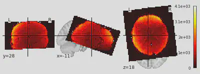
4. Plot data of one example participant
data_one = fetch_data(n_subjects=1)
fmri_filename = "nilearn_data/sub-pixar016_func_sub-pixar016_task-pixar_bold.nii"
conf = "nilearn_data/derivatives_preprocessed_data_sub-pixar016_sub-pixar016_task-pixar_run-001_ART_and_CompCor_nuisance_regressors.mat"
averaged_Img = image.mean_img(image.mean_img(myImg))
plotting.plot_stat_map(averaged_Img)
<nilearn.plotting.displays.OrthoSlicer at 0x7fd96c2b6050>
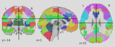
5. Plotting and preparing brain atlas parcellation
parcellations = datasets.fetch_atlas_basc_multiscale_2015(version='sym')
atlas_filename = parcellations.scale064
plotting.plot_roi(atlas_filename)

print('Atlas ROIs are located in nifti image (4D) at: %s' %
       atlas_filename)

multiscale = datasets.fetch_atlas_basc_multiscale_2015()
atlas_filename = multiscale.scale064

# initialize masker (change verbosity)
masker = NiftiLabelsMasker(labels_img=atlas_filename, standardize=True,
                           memory='nilearn_cache', verbose=0)
# initialize correlation measure, set to vectorize
correlation_measure = ConnectivityMeasure(kind='correlation', vectorize=True,
                                         discard_diagonal=True)
Atlas ROIs are located in nifti image (4D) at: /home/mjovanova@asc.upenn.edu/nilearn_data/basc_multiscale_2015/template_cambridge_basc_multiscale_nii_sym/template_cambridge_basc_multiscale_sym_scale064.nii.gz
6. Create confounds function
def prepare_confounds(conf, key = 'R', transpose=True):
    arrays = {}
    f = h5py.File(conf)
    for k, v in f.items():
        arrays[k] = np.array(v)

    if transpose:
        output = arrays[key].T
    else:
        output = arrays[key]

    return output
7. Mask time series data and apply confound regression
#load files for one individual
fmri_filename = "nilearn_data/sub-pixar016_func_sub-pixar016_task-pixar_bold.nii"
conf = "nilearn_data/derivatives_preprocessed_data_sub-pixar016_sub-pixar016_task-pixar_run-001_ART_and_CompCor_nuisance_regressors.mat"
conf = prepare_confounds(conf) #apply confounds function
time_series = masker.fit_transform(myImg,confounds=conf)#apply mask
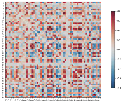
7. Run correlations and plot time series correlation matrix for one individual
correlation_measure = ConnectivityMeasure(kind='correlation')
correlation_matrix = correlation_measure.fit_transform([time_series])[0]
#correlation_matrix.shape
# Mask the main diagonal for visualization:
np.fill_diagonal(correlation_matrix, 0)

# The labels we have start with the background (0), hence we skip the
# first label
plotting.plot_matrix(correlation_matrix, figure=(10, 8),
                     labels=range(time_series.shape[-1]),
                     vmax=0.8, vmin=-0.8, reorder=False)
<matplotlib.image.AxesImage at 0x7fd96bfcedd0>
Part 2. Apply machine-learning tools for prediction
As a working example, we will try to predict participant age based on their brain connectivity signals while watching the Pixar movie.
1. Load participant phenotype data
data.phenotypic
pheno = pd.DataFrame(data.phenotypic, columns =['participant_id', 'Age', 'Child_Adult', 'AgeGroup']) #save varaibles we need as pandas df
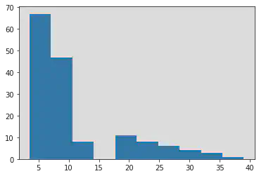
2. Inspect outcome age variable
y_age = pheno['Age']
y_age.head()
plt.hist(y_age)
#Seems pretty skewed toward younger children and we may log-transform age.
(array([67., 47.,  8.,  0., 11.,  8.,  6.,  4.,  3.,  1.]),
 array([ 3.51813826,  7.06632443, 10.61451061, 14.16269678, 17.71088296,
        21.25906913, 24.8072553 , 28.35544148, 31.90362765, 35.45181383,
        39.        ]),
 <BarContainer object of 10 artists>)
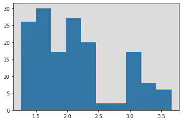
log_y_age = np.log(y_age)
plt.hist(log_y_age)
(array([26., 30., 17., 27., 20.,  2.,  2., 17.,  8.,  6.]),
 array([1.25793195, 1.49849492, 1.73905789, 1.97962086, 2.22018383,
        2.4607468 , 2.70130977, 2.94187274, 3.18243571, 3.42299868,
        3.66356165]),
 <BarContainer object of 10 artists>)
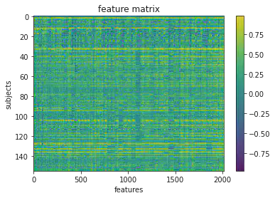
3. Load brain features
feat_file = 'nilearn_data/BASC064_features.npz'
X_features = np.load(feat_file)['a']
plt.imshow(X_features, aspect='auto')
plt.colorbar()
plt.title('feature matrix')
plt.xlabel('features')
plt.ylabel('subjects')
Text(0, 0.5, 'subjects')
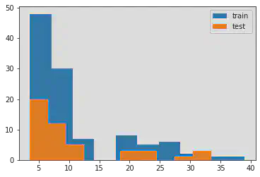
4. Prep data and split into train and testing samples (70/30 split)
age_groups = pheno['AgeGroup'] #prep variable to stratify folds by age groups
# Split the sample to training/test with a 60/40 ratio, and
# stratify by age group, and also shuffle the data.

X_train, X_test, y_train, y_test, ageGroup_train, ageGroup_test = train_test_split(
                                                                X_features,
                                                                y_age,
                                                                age_groups,
                                                                test_size = 0.3,
                                                                shuffle = True,
                                                                stratify = age_groups,
                                                                random_state = 123
                                                                                   )

# print the size of our training and test groups
print('training:', len(X_train),
     'testing:', len(X_test))
training: 108 testing: 47
plt.hist(y_train, label = 'train')
plt.hist(y_test, label = 'test')
plt.legend()
<matplotlib.legend.Legend at 0x7fd96bb11510>
5. Fit linear model
l_svr = SVR(kernel='linear') # define the model
l_svr.fit(X_train, y_train) # fit the model
SVR(C=1.0, cache_size=200, coef0=0.0, degree=3, epsilon=0.1, gamma='scale',
    kernel='linear', max_iter=-1, shrinking=True, tol=0.001, verbose=False)
y_pred = l_svr.predict(X_train) # predict the training data based on the model
r2 = l_svr.score(X_train, y_train) # get the r2
mae = mean_absolute_error(y_true = y_train,
                          y_pred = y_pred) # get the mae
6. Tranform data
log_y_train = np.log(y_train) # log-transform target data based on training distribution
transformer = FunctionTransformer(np.log).fit(y_train.values.reshape(-1,1))
log_y_test = transformer.transform(y_test.values.reshape(-1,1))[:,0]
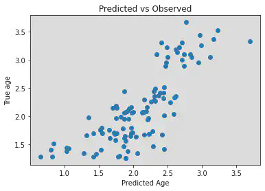
7. Refit model and assess performance
y_pred = cross_val_predict(l_svr, X_train, log_y_train, groups=ageGroup_train, cv=5)
r2 = cross_val_score(l_svr, X_train, log_y_train, groups=ageGroup_train, cv=5)
mae_score = cross_val_score(l_svr, X_train, log_y_train, groups=ageGroup_train, cv=5,
                           scoring = 'neg_mean_absolute_error')

# don't forget to switch y_train to log_y_train
overall_r2 = r2_score(y_pred = y_pred, y_true = log_y_train)
overall_mae = mean_absolute_error(y_pred = y_pred, y_true = log_y_train)
print('r2 = %s, mae = %s'%(overall_r2,overall_mae))

plt.scatter(y_pred, log_y_train)
plt.title('Predicted vs Observed')
plt.xlabel('Predicted Age')
plt.ylabel('True age')
r2 = 0.6293239920471065, mae = 0.3093765475577604


Text(0, 0.5, 'True age')
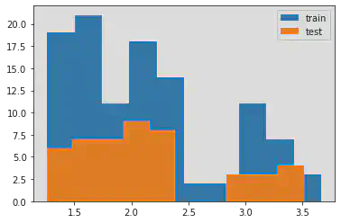
8. Plot training vs. test samples data
plt.hist(log_y_train, label = 'train')
plt.hist(log_y_test, label = 'test')
plt.legend()
<matplotlib.legend.Legend at 0x7fd96b9c1090>
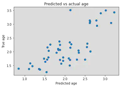
9. Test model performance on test set
l_svr.fit(X_train, log_y_train) # fit to training data
y_pred = l_svr.predict(X_test) # predict age using testing data
r2 = l_svr.score(X_test, log_y_test) # get r2 score
mae = mean_absolute_error(y_pred=y_pred, y_true=log_y_test) # get mae

# print results
print('r2 = %s, mae = %s'%(r2,mae))

# plot results
plt.scatter(y_pred, log_y_test)
plt.title('Predicted vs actual age')
plt.xlabel('Predicted age')
plt.ylabel('True age')
r2 = 0.5545446467557136, mae = 0.3545248009510429


Text(0, 0.5, 'True age')
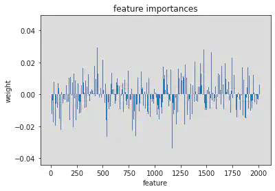
9. Preliminary plot of feature importance in the brain
plt.bar(range(l_svr.coef_.shape[-1]),l_svr.coef_[0])
plt.title('feature importances')
plt.xlabel('feature')
plt.ylabel('weight')
Text(0, 0.5, 'weight')